|
|
|
Архитектура Астрономия Аудит Биология Ботаника Бухгалтерский учёт Войное дело Генетика География Геология Дизайн Искусство История Кино Кулинария Культура Литература Математика Медицина Металлургия Мифология Музыка Психология Религия Спорт Строительство Техника Транспорт Туризм Усадьба Физика Фотография Химия Экология Электричество Электроника Энергетика |
Із рівнянь (5.8) – (5.9) знаходимо
Підстановка (5.7) і (5.10) в (5.5) після піднесення (5.5) до квадрату дає
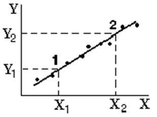
де а Таким чином, залежність Y = f(X) за теорією повинна бути лінійною. Експериментально досліджується залежність між періодом коливань Т фізичного маятника та відстанню Z вантажу до точки підвісу. Будується графік у координатах Y = f(X). Якщо одержується прямолінійний графік, то це підтверджує справедливість теоретичних формул (5.5) і (5.7), а по нахилу графіка можна розрахувати прискорення вільного падіння g. Співпадання його з табличним значенням 9,8 м/с2 кількісно підтверджує справедливість теоретичних співвідношень.
Практична частина
1. Увімкнути вилку живлення приладу в мережу 220 В і натиснути кнопку „СЕТЬ”. 2. Зняти маятник з кронштейна 6, відпустити фіксатор 9 і встановити центр вантажу 8 на відстані 10 см від точки підвісу. Відстань вимірювати кількістю видимих кільцевих нарізок на стержні від опорної призми (точки підвісу) до вантажу плюс 1 см, що враховує товщину вантажу (2 см). Добиватись чіткої фіксації вантажу в нарізках. 3. Підвісити маятник на кронштейн 6. При цьому слідкувати за надійністю його кріплення, щоб опорна призма чітко потрапила у заглиблення. 4. Відрегулювати положення кронштейна 4 так, щоб нижній кінець стержня маятника 7 не зачіпався за фотоелектричний датчик 5, але перекривав його промінь. 5. Привести маятник у коливання, відхиливши його на кут не більший, ніж 5о. 6. Після того, як маятник здійснить 1 ÷ 2 коливання, натиснути кнопку “СБРОС”. Почнеться відлік часу та кількості коливань, що буде видно на відповідних індикаторах. 7. Коли на індикаторі кількості коливань появиться цифра 9, натиснути кнопку “СТОП”. Після закінчення останнього 10-го коливання зупиниться секундомір. 8. Визначити період коливань, поділивши час на кількість коливань, тобто на 10. Відстань Z та період Т записати в таблицю 5.1.
Таблиця 5.1
9. Повторювати пп. 2 ÷ 8, кожного разу переміщувати вантаж вниз на 2 см (по дві нарізки) до найнижчого можливого положення. 10. За формулою (5.12) розрахувати Х і записати в таблицю 5.1. 11. Побудувати графік залежності Y=f(X). 12. На прямолінійній його частині вибрати дві точки 1 і 2, (рис.5.4) визначити їх координати по осям, але не із таблиці, і знайти прискорення вільного падіння за формулою
13. Порівняти одержане значення з довідковим 980 см/с2. Зробити висновок.
Контрольні запитання
1. Що таке фізичний маятник? 2. Складіть та запишіть диференціальне рівняння вільних гармонічних коливань фізичного маятника. 3. Запишіть рівняння коливань, яке є розв’язком диференціального рівняння фізичного маятника. Накресліть графік цього рівняння. 4. Як називають величини, що входять в рівняння коливань фізичного маятника. Які розмірності цих величин? 5. Запишіть формули для періоду та циклічної частоти коливань фізичного маятника.
Література
1. Чолпан П.П. Фізика.- К.: Вища школа, 2003.- С.77-80. 2. Савельев И.В. Курс общей физики. - т.1, М.: Наука,1982.- С.196-199. 3. Трофимова Т.И. Курс физики.- М: Высшая школа, 1990.- С.222-223.
Інструкцію склав доцент каф. фізики ЗНТУ Манько В.К.
6 LABORATORY Work № 43.1 PHYSICAL PENDULUM Purpose of work:check the dependence of physical pendulum free oscillations period from its moment of inertia; determine the value of the free fall acceleration. DEVICES AND EQUIPMENT: physical pendulum, stopwatch, straightedge.
The experimental setting(fig.6.1)consists of the base 1, alignment of which is carried out by legs 2. The rack is fastened in the base 3, on which the bottom supporting arm 4 is fixed with photoelectric sensor 5. On the top supporting arm 6 is suspended the physical pendulum, which includes the rod 7, weight 8 and detent 9. On the rod 7 in 10 mm collar marks are made for the exact determination of the length and exact weight 8 fixation. On the front gage panel there are: 10 – oscillation indicator, 14 – indicator of time, switches: -11 “Сеть”, 12 “Сброс”, 13 “Стоп”.
During the pendulum motion the flow of light from the lamp of the photoelectric sensor overlap and the electronic computation circuit of oscillations number and stopwatch actuates. After pressing the switch “STOP” the stopwatch stanching after the end of full current oscillations. Theoretical part
Physical pendulum – is the solid, which can rotate relatively to the arbitrary of the horizontal axis that doesn’t pass through the center of mass. Moment of the gravity force mg, the arm of which is equal L·sin α. Value of L is the distance from pivot О (suspension center) to point С – the center of the mass of the body. Under the action of this moment the body turns round the suspension centerО.
Figure 6.2
Write down the fundamental equation of the rotational motion dynamics
where I is the moment of inertia of the body,
If angle α is small (less than 5о) we can consider that sin α = α. We get
Figure 6.3 The moment of inertia of the pendulum relatively to the point О is equal to the amount of moment of inertia of the load and rod.
Taking into account Steiner theorem, we obtain
Thus, the moment of inertia of the pendulum as function of distance Z from point of suspension to weight center
From figure 3 we can see that
where
а
Thus, dependence Y = f(X) according to the theory, must be linear. Experimentally researched is the dependence of oscillations period Т of physical pendulum and distance Z from weight to suspension center. We plot the graph (6.12) Y=f(X). If you get a rectilinear graph, it confirms validity of theoretical formulas (6.5) and (6.7), and on its slope we can find the free fall acceleration g. Its coincidence with tabulated value 9,8 m/s2 confirms truth of the theoretical ratio.
Work procedure
1. Connect a device to the mains 220 V and push the button „Сеть”. 2. Remove the pendulum from the support arm 6, release the detent 9 and station the weight 8 center on the distance 10 сm from the suspension point. Measure the distance with the number of known collar marks on the rod from supportive prisms (suspension center) plus 1 сm to the weight which includes the thickness of the load (2 sm). Seek a clear fixing of a load in marks. 3. Hang up the pendulum on the supportive arm 6. Watch after its mounting reliability. 4. Regulate the supportive arm 4 position so that the bottom rod end of physical pendulum 7 won’t catch on photoelectric sensor 5, but block its ray. 5. Activate physical pendulum in oscillations, having rejected it on a corner less than 5о. 6. After the pendulum make 1 ÷ 2 oscillations, push the button “Сброс”. Counting of time and oscillations number will start which will be visible on corresponding indicators. 7. When oscillations indicator shows up number 9, press the button “Стоп”. The last 10-th oscillation will finish and the stopwatch will stop. 8. Define the period of oscillations, dividing time for oscillations number that is 9. Distance Z and period Т write down to the table. 9. Repeat points 2÷8, removing the weight down in 2 cm to the possibly lowest weight position. 10. Under formula (6.12) calculate Х and write it down to the table. Pendulum parameters are: mass ratio 11. Plot the dependence Y = f(X) and choose two points 1 and 2 on its rectilinear part and define its coordinate by axes, not from the table, on the graph inclination find the free fall acceleration by the formula
Table 6.1
Figure 6.4
Control questions
6. What is the physical pendulum? 7. Deduce and write down the differential equation of physical pendulum’s free harmonic oscillations. 8. Write down the oscillations equation which is the solution of physical pendulum differential equation. Plot the graph of this equation. 9. What is the name of values which are a part of physical pendulum oscillations equation? What units they have? 10. Write down formulas for period and physical pendulum’s cyclic oscillation frequency.
Literature
1. Чолпан П.П. Фізика.- К.: Вища школа, 2003.- С.77-80. 2. Савельев И.В. Курс общей физики. - т. 1, М.: Наука,1982.- С.196-199. 3. Трофимова Т.И. Курс физики.- М: Высшая школа, 1990.- С.222-223.
Translator: S.P. Lushchin, the reader, candidate of physical and mathematical sciences. Reviewer: S.V. Loskutov, professor, doctor of physical and mathematical sciences.
Approved by the chair of physics. Protocol № 6 from 30.03.2009 .
Поиск по сайту: |
 (5.10)
 , (5.11)
 ,
,  ,
,
 . (5.12)
 Параметри маятника: відношення мас m/M = 0,3; довжина верхнього кінця стержня до точки підвісу а = 5 см; загальна довжина стержня b = 59 см. Розрахунки зручніше виконувати на ЕОМ.
 , см/с2. (5.13)

 ,(6.1)
 is angular acceleration, minus accounts that the moment of force of mg reduces the angle α.Thus, we get the differential equation of physical pendulum free oscillations
 . (6.2)
 . (6.3) Comparing the received equation with the general equation of free harmonic oscillations
 , (6.4) where
  - is cyclic frequency of oscillations, Т – period. Let’s get the equation of the period of oscillations
 . (6.5) Equation solution (6.4) is the harmonic function which is the equation of free harmonic oscillations
 . (6.6) For performing the first task point we need to change the moment of inertia of the pendulum. It is carried out by moving the weight 8 along the rod 7. But in this way the mass center position changes, it is the distance L.

 .
. . (6.7) Let’s find the position of point С the mass center of pendulum which is the distance L as function Z. By the law of moments relatively to the point C we have:
 . (6.8)
 ,
,  . (6.9) From equations (6.8) – (6.9) we get
 . (6.10) Substitution of (6.7) and (6.10) into (6.5) after squaring (6.5) gives us
 , (6.11)
 ,
, ,
, . (6.12)
 0,3; Length of the bottom rod end to suspension point а = 5 cm; total rod length b = 59 cm. Calculation it is more convenient to do on the computer.
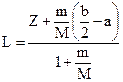
 , cm/s2. (6.13) Compare the received value with reference 980 cm/s2. Write the conclusion.