Experimental setting description

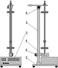
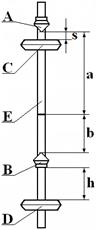
The experimental setting is represented on a fig. 12.1. On a vertical column 1, which is set on the basis of 2 with the electronic stop-watch 3 located on him, two brackets are fixed: lower mobile 4 with the photo-electric sensor 5 and overhead immobile 6. On an overhead immobile bracket 6 a circulating pendulum which is a steel rod E on which supporting prisms A and B and mobile weights C and D are fixed is suspended (fig. 12.2).

Figure 12.1

Figure 12.2

Theoretical part

In any physical pendulum it is possible to find such two points on its ax, that at the successive fixing of pendulum in a that or other point the period of oscillations of the pendulum will remain unchanging. In our case of circulating pendulum these two points is the position of prisms A and B (fig. 12.2). At fixing of circulating pendulum by prisms A and B by moving of weights C and D along its axis it is possible to obtain equality of periods of its oscillations:

(12.1)

where I_A and I_B are moments of inertia of pendulum in relation to axes which pass through the points of A and B; a and b is distance from the centre of gravity to the proper ax of oscillations. On the basis of Steiner theorem:

, (12.2)

where I₀ is a moment of inertia of pendulum in relation to an ax which passes through its centre of gravity and which is parallel to an ax of oscillations.

Putting (12.2) in (12.1), we will get a formula for calculation of gravity acceleration g:

(12.3)

The value L=a+b, which is equal to distance between prisms, called the equivalent length of physical pendulum. Thus, for determination of gravity acceleration by a circulating pendulum it is necessary to measure two values: the equivalent length L and the period of oscillations T=T_A=T_B of physical pendulum.

Practical part

1. Insert the power cord of device into a network and push the button "Сеть".

2. Check up the work of indicators and bulbs of photo-electric sensor: the indicators of electronic stop-watch and meter of amount of oscillations (periods) must shine "0" in all of digits, and bulb of photo-electric sensor to shine.

3. Fix the weight C on the distance s=5+n сm (where n is a number of educational brigade) from the prism A, and the weight D – in the distance h=1 cm from the prism B (fig. 12.2).

4. Find the distance L between prisms, using a scale which is inflicted on a rod.

5. Fix the pendulum on liner of overhead bracket of setting on the prism A.

6. Displace the lower bracket of setting so that the rod of pendulum crossed the optical axis of photo-electric sensor.

7. Decline a pendulum from a position of equilibrium on a corner of 5-10° and enable it to carry out free oscillations.

8. Push the button "Сброс".

9. Measure the time of N=10 of full pendulum oscillations, for what after the count of 9 full oscillations push the button "Стоп" on the stop-watch.

10. Calculate the pendulum oscillations period T using the formula:

(12.4)

where t is the total time of N oscillations.

11. For different positions h of weight D on the rod of pendulum count up the period of oscillations T_A in accordance to points 7-10. Change the position of weight D on the rod of pendulum through every basic scale division, that is through 1 sm. Thus the position of weight C remains constant. Enter the results of measurements to the table 12.1.

Table 12.1

12. Hang up the pendulum on a prism B.

13. Lift the lower bracket with the photoelectric sensor according to p. 6.

14. Determine the period T_B of oscillations of the pendulum for different positions of weight D on the rod E in those limits and with the same number of measurements. Put down the results of measurements to the table 12.1.

15. According to table 12.1 draw the graphs of oscillation periods T_A and T_B from the position h of weight D on the pendulum rod: T_A=f(h) and T_B=f(h). Intersection of curves will determine the position of movable weight D on the pendulum rod, at which the values of periods will be equal Т_A=Т_B=T.

16. Find pendulum oscillations periods for this weight D position according to points 7÷10 relatively to prisms A and B. The measurement of oscillation periods relatively to each prism perform 3 times. Enter the results of measurements to the table 12.2:

17. Calculate the pendulum oscillations period using the formula:

(12.5)

18. Calculate the gravity acceleration using the formula (12.3). Submit the result in a following form:

where Δg – absolute error of g, which can be found from the formula:

(12.6)

Δπ is calculated as the error of tabular value; ΔL – as the error of direct unit measurement.

Absolute error of measurement of can be found using the formula:

(12.7)

where ΔT_A, ΔT_B are defined as the errors of multiple direct measurements.

19. Compare the got experimental value to theoretical value m/sec².

20. Write a conclusion.

Table 12.2

№	с	с	,с2	с	с	с2
	, с	—	, c2	, с	—	, с2

Control questions

1. What is the gravity acceleration? What is the direction of gravity acceleration and on what it depends?

2. Define the physical pendulum.

3. Deduce a formula for the physical pendulum oscillations period.

4. Define a physical pendulum reduced value?

5. State the Steiner theorem.

Authors: S.V. Seidametov, senior lecturer.

Reviewer: S.V. Loskutov, professor, doctor of physical and mathematical sciences.

Approved by the chair of physics. Protocol № 6 from 30.03.2009.

Поиск по сайту: